My Blog: Sampling

Load r packages

library(tidyverse)
library(moderndive)

Modify the code for comparing different sample sizes from the virtual bowl

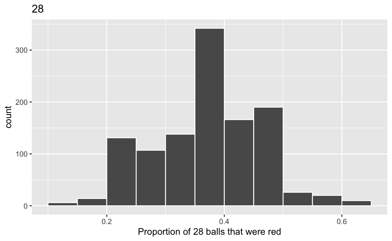
#Segment 1: sample size = 28

1.a) Take 1150 samples of size of 28 instead of 1000 replicates of size 25 from the bowl dataset. Assign the output to virtual_samples_28

virtual_samples_28  <- bowl  %>% 
rep_sample_n(size = 28, reps = 1150)

1.b) Compute resulting 1150 replicates of proportion red

start with virtual_samples_28 THEN group_by replicate THEN create variable red equal to the sum of all the red balls create variable prop_red equal to variable red / 28 Assign the output to virtual_prop_red_28

virtual_prop_red_28 <- virtual_samples_28 %>% 
  group_by(replicate) %>% 
  summarize(red = sum(color == "red")) %>% 
  mutate(prop_red = red / 28)

1.c) Plot distribution of virtual_prop_red_28 via a histogram

use labs to

label x axis = “Proportion of 28 balls that were red” create title = “28”

ggplot(virtual_prop_red_28, aes(x = prop_red)) +
  geom_histogram(binwidth = 0.05, boundary = 0.4, color = "white") +
  labs(x = "Proportion of 28 balls that were red", title = "28")

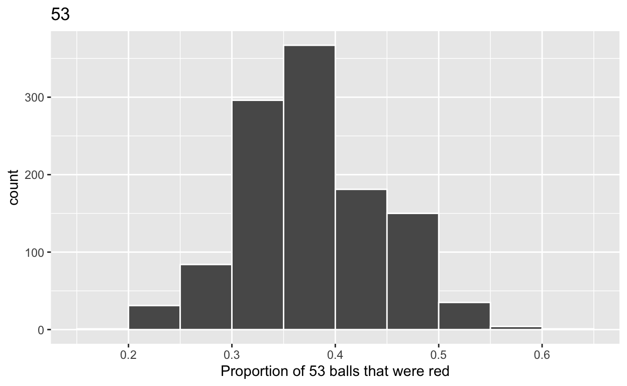
#Segment 2: sample size = 53

2.a) Take 1150 samples of size of 53 instead of 1000 replicates of size 50. Assign the output to virtual_samples_53

virtual_samples_53 <- bowl  %>% 
rep_sample_n(size = 53, reps = 1150)

2.b) Compute resulting 1150 replicates of proportion red

start with virtual_samples_53 THEN group_by replicate THEN create variable red equal to the sum of all the red balls create variable prop_red equal to variable red / 53 Assign the output to virtual_prop_red_53

virtual_prop_red_53 <- virtual_samples_53 %>% 
  group_by(replicate) %>% 
  summarize(red = sum(color == "red")) %>% 
  mutate(prop_red = red / 53)

2.c) Plot distribution of virtual_prop_red_53 via a histogram

use labs to

label x axis = “Proportion of 53 balls that were red” create title = “53”

ggplot(virtual_prop_red_53, aes(x = prop_red)) +
  geom_histogram(binwidth = 0.05, boundary = 0.4, color = "white") +
  labs(x = "Proportion of 53 balls that were red", title = "53")

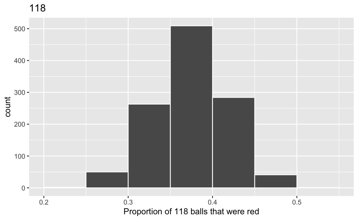
#Segment 3: sample size = 118

3.a) Take 1150 samples of size of 118 instead of 1000 replicates of size 50. Assign the output to virtual_samples_118

virtual_samples_118  <- bowl  %>% 
rep_sample_n(size = 118, reps = 1150)

3.b) Compute resulting 1150 replicates of proportion red

start with virtual_samples_118 THEN group_by replicate THEN create variable red equal to the sum of all the red balls create variable prop_red equal to variable red / 118 Assign the output to virtual_prop_red_118

virtual_prop_red_118 <- virtual_samples_118 %>% 
  group_by(replicate) %>% 
  summarize(red = sum(color == "red")) %>% 
  mutate(prop_red = red / 118)

3.c) Plot distribution of virtual_prop_red_118 via a histogram

use labs to

label x axis = “Proportion of 118 balls that were red” create title = “118”

ggplot(virtual_prop_red_118, aes(x = prop_red)) +
  geom_histogram(binwidth = 0.05, boundary = 0.4, color = "white") +
  labs(x = "Proportion of 118 balls that were red", title = "118")

Calculate the standard deviations for your three sets of 1150 values of prop_red using the standard deviation

n = 28

virtual_prop_red_28  %>% 
  summarize(sd = sd(prop_red))

# A tibble: 1 x 1
      sd
   <dbl>
1 0.0899

n = 53

virtual_prop_red_53  %>% 
  summarize(sd = sd(prop_red))

# A tibble: 1 x 1
      sd
   <dbl>
1 0.0667

n = 118

virtual_prop_red_118  %>% 
  summarize(sd = sd(prop_red))

# A tibble: 1 x 1
      sd
   <dbl>
1 0.0436

The distribution with sample size, n = 118, has the smallest standard deviation (spread) around the estimated proportion of red balls.