Steps 1-6
- Load the R packages we will use
- Read the data in the files
drug_cos <- read_csv("https://estanny.com/static/week6/drug_cos.csv")
health_cos <- read_csv("https://estanny.com/static/week6/health_cos.csv")
- Use ‘glimpse’ to get a glimpse of the data
drug_cos %>% glimpse()
Rows: 104
Columns: 9
$ ticker       <chr> "ZTS", "ZTS", "ZTS", "ZTS", "ZTS", "ZTS", "ZTS…
$ name         <chr> "Zoetis Inc", "Zoetis Inc", "Zoetis Inc", "Zoe…
$ location     <chr> "New Jersey; U.S.A", "New Jersey; U.S.A", "New…
$ ebitdamargin <dbl> 0.149, 0.217, 0.222, 0.238, 0.182, 0.335, 0.36…
$ grossmargin  <dbl> 0.610, 0.640, 0.634, 0.641, 0.635, 0.659, 0.66…
$ netmargin    <dbl> 0.058, 0.101, 0.111, 0.122, 0.071, 0.168, 0.16…
$ ros          <dbl> 0.101, 0.171, 0.176, 0.195, 0.140, 0.286, 0.32…
$ roe          <dbl> 0.069, 0.113, 0.612, 0.465, 0.285, 0.587, 0.48…
$ year         <dbl> 2011, 2012, 2013, 2014, 2015, 2016, 2017, 2018…
health_cos %>% glimpse()
Rows: 464
Columns: 11
$ ticker      <chr> "ZTS", "ZTS", "ZTS", "ZTS", "ZTS", "ZTS", "ZTS"…
$ name        <chr> "Zoetis Inc", "Zoetis Inc", "Zoetis Inc", "Zoet…
$ revenue     <dbl> 4233000000, 4336000000, 4561000000, 4785000000,…
$ gp          <dbl> 2581000000, 2773000000, 2892000000, 3068000000,…
$ rnd         <dbl> 427000000, 409000000, 399000000, 396000000, 364…
$ netincome   <dbl> 245000000, 436000000, 504000000, 583000000, 339…
$ assets      <dbl> 5711000000, 6262000000, 6558000000, 6588000000,…
$ liabilities <dbl> 1975000000, 2221000000, 5596000000, 5251000000,…
$ marketcap   <dbl> NA, NA, 16345223371, 21572007994, 23860348635, …
$ year        <dbl> 2011, 2012, 2013, 2014, 2015, 2016, 2017, 2018,…
$ industry <chr> "Drug Manufacturers - Specialty & Generic", "Dr…- Which variables are the same in both data sets
names_drug <- drug_cos %>% names()
names_health <- health_cos %>% names()
intersect(names_drug, names_health)
[1] "ticker" "name" "year" - Select subset of variables to work with
drug_subset <- drug_cos %>%
  select(ticker, year, grossmargin) %>%
  filter(year == 2018)
health_subset <- health_cos %>%
  select(ticker, year, gp, industry) %>%
  filter(year == 2018)
- Keep all the rows and columns drug_subset join with columns in health_subset
drug_subset %>% left_join(health_subset)
# A tibble: 13 x 5
   ticker  year grossmargin         gp industry
   <chr>  <dbl>       <dbl>      <dbl> <chr>
 1 ZTS     2018       0.672    3.91e 9 Drug Manufacturers - Specialty…
 2 PRGO    2018       0.387    1.83e 9 Drug Manufacturers - Specialty…
 3 PFE     2018       0.79     4.24e10 Drug Manufacturers - General
 4 MYL     2018       0.35     4.00e 9 Drug Manufacturers - Specialty…
 5 MRK     2018       0.681    2.88e10 Drug Manufacturers - General
 6 LLY     2018       0.738    1.81e10 Drug Manufacturers - General
 7 JNJ     2018       0.668    5.45e10 Drug Manufacturers - General
 8 GILD    2018       0.781    1.73e10 Drug Manufacturers - General
 9 BMY     2018       0.71     1.60e10 Drug Manufacturers - General
10 BIIB    2018       0.865    1.16e10 Drug Manufacturers - General
11 AMGN    2018       0.827    1.96e10 Drug Manufacturers - General
12 AGN     2018       0.861    1.36e10 Drug Manufacturers - General
13 ABBV    2018       0.764    2.50e10 Drug Manufacturers - General
Question: join_ticker
Start with drug_cos
Extract observations for the ticker JNJ from drug_cos Assign output to the variable drug_cos_subset
drug_cos_subset <- drug_cos %>%
 filter(ticker == "JNJ")
Display drug_cos_subset
drug_cos_subset
# A tibble: 8 x 9
  ticker name  location ebitdamargin grossmargin netmargin   ros   roe
  <chr>  <chr> <chr>           <dbl>       <dbl>     <dbl> <dbl> <dbl>
1 JNJ    John… New Jer…        0.247       0.687     0.149 0.199 0.161
2 JNJ    John… New Jer…        0.272       0.678     0.161 0.218 0.173
3 JNJ    John… New Jer…        0.281       0.687     0.194 0.224 0.197
4 JNJ    John… New Jer…        0.336       0.694     0.22  0.284 0.217
5 JNJ    John… New Jer…        0.335       0.693     0.22  0.282 0.219
6 JNJ    John… New Jer…        0.338       0.697     0.23  0.286 0.229
7 JNJ    John… New Jer…        0.317       0.667     0.017 0.243 0.019
8 JNJ    John… New Jer…        0.318       0.668     0.188 0.233 0.244
# … with 1 more variable: year <dbl>
Use left join to combine the rows and columns of drug_cos_subset with the columns of health_cos
Assign the output to combo_df
combo_df <- drug_cos_subset %>%
  left_join(health_cos)
Display combo_df
combo_df
# A tibble: 8 x 17
  ticker name  location ebitdamargin grossmargin netmargin   ros   roe
  <chr>  <chr> <chr>           <dbl>       <dbl>     <dbl> <dbl> <dbl>
1 JNJ    John… New Jer…        0.247       0.687     0.149 0.199 0.161
2 JNJ    John… New Jer…        0.272       0.678     0.161 0.218 0.173
3 JNJ    John… New Jer…        0.281       0.687     0.194 0.224 0.197
4 JNJ    John… New Jer…        0.336       0.694     0.22  0.284 0.217
5 JNJ    John… New Jer…        0.335       0.693     0.22  0.282 0.219
6 JNJ    John… New Jer…        0.338       0.697     0.23  0.286 0.229
7 JNJ    John… New Jer…        0.317       0.667     0.017 0.243 0.019
8 JNJ    John… New Jer…        0.318       0.668     0.188 0.233 0.244
# … with 9 more variables: year <dbl>, revenue <dbl>, gp <dbl>,
#   rnd <dbl>, netincome <dbl>, assets <dbl>, liabilities <dbl>,
#   marketcap <dbl>, industry <chr>
Note: the variables ticker, name , location, and industry are the same for all the observations
Assign the company name to co_name’
co_name <- combo_df %>%
  distinct(name) %>%
  pull()
Assign the company location to co_location
co_location <- combo_df %>%
  distinct(location) %>%
  pull()
Assign the industry to co_industry group
co_industry <- combo_df %>%
  distinct(location) %>%
  pull()
Start with the combo_df
Select variables(in this order): year, grossmargin, netmargin, revenue, gp, netincome
Assign the output to combo_df_subset
combo_df_subset <- combo_df %>%
  select(year, grossmargin, netmargin, revenue, gp, netincome)
Display combo_df_subset
combo_df_subset
# A tibble: 8 x 6
   year grossmargin netmargin     revenue          gp   netincome
  <dbl>       <dbl>     <dbl>       <dbl>       <dbl>       <dbl>
1  2011       0.687     0.149 65030000000 44670000000  9672000000
2  2012       0.678     0.161 67224000000 45566000000 10853000000
3  2013       0.687     0.194 71312000000 48970000000 13831000000
4  2014       0.694     0.22  74331000000 51585000000 16323000000
5  2015       0.693     0.22  70074000000 48538000000 15409000000
6  2016       0.697     0.23  71890000000 50101000000 16540000000
7  2017       0.667     0.017 76450000000 51011000000  1300000000
8  2018       0.668     0.188 81581000000 54490000000 15297000000
Create the variable grossmargin_check to compare with the variable grossmargin. They should be equal. grossmargin_check = gp / revenue
Create the variable close_enough to check that the absolute value of the difference between grossmargin_check and grossmargin is less than 0.001
combo_df_subset %>%
  mutate(grossmargin_check = gp/revenue,
  close_enough = abs(grossmargin_check - grossmargin) < 0.001)
# A tibble: 8 x 8
   year grossmargin netmargin revenue      gp netincome
  <dbl>       <dbl>     <dbl>   <dbl>   <dbl>     <dbl>
1  2011       0.687     0.149 6.50e10 4.47e10   9.67e 9
2  2012       0.678     0.161 6.72e10 4.56e10   1.09e10
3  2013       0.687     0.194 7.13e10 4.90e10   1.38e10
4  2014       0.694     0.22  7.43e10 5.16e10   1.63e10
5  2015       0.693     0.22  7.01e10 4.85e10   1.54e10
6  2016       0.697     0.23  7.19e10 5.01e10   1.65e10
7  2017       0.667     0.017 7.64e10 5.10e10   1.30e 9
8  2018       0.668     0.188 8.16e10 5.45e10   1.53e10
# … with 2 more variables: grossmargin_check <dbl>,
#   close_enough <lgl>
Create the variable netmargin_check to compare with the variable netmargin. They should be equal.
Create the variable close_enough to check that the absolute value of the difference between netmargin_check and netmargin is less than 0.001
combo_df_subset %>%
  mutate(netmargin_check = netincome/revenue,
  close_enough = abs(netmargin_check - netmargin) < 0.001)
# A tibble: 8 x 8
   year grossmargin netmargin revenue      gp netincome
  <dbl>       <dbl>     <dbl>   <dbl>   <dbl>     <dbl>
1  2011       0.687     0.149 6.50e10 4.47e10   9.67e 9
2  2012       0.678     0.161 6.72e10 4.56e10   1.09e10
3  2013       0.687     0.194 7.13e10 4.90e10   1.38e10
4  2014       0.694     0.22  7.43e10 5.16e10   1.63e10
5  2015       0.693     0.22  7.01e10 4.85e10   1.54e10
6  2016       0.697     0.23  7.19e10 5.01e10   1.65e10
7  2017       0.667     0.017 7.64e10 5.10e10   1.30e 9
8  2018       0.668     0.188 8.16e10 5.45e10   1.53e10
# … with 2 more variables: netmargin_check <dbl>, close_enough <lgl>
Question: summarize_industry
Fill in the blanks
Put the command you use in the Rchunks in the Rmd file for this quiz
Use the health_cos data
For each industry calculate
mean_grossmargin_percent = mean(gp / revenue) * 100 median_grossmargin_percent = median(gp / revenue) * 100 min_grossmargin_percent = min(gp / revenue) * 100 max_grossmargin_percent = max(gp / revenue) * 100
health_cos %>%
  group_by(industry) %>%
  summarize(mean_grossmargin_percent = mean(gp / revenue) * 100,
median_grossmargin_percent = median(gp / revenue) * 100,
min_grossmargin_percent = min(gp / revenue) * 100,
max_grossmargin_percent = max(gp / revenue) * 100)
# A tibble: 9 x 5
  industry mean_grossmargi… median_grossmar… min_grossmargin…
* <chr>               <dbl>            <dbl>            <dbl>
1 Biotech…             92.5            92.7             81.7
2 Diagnos…             50.5            52.7             28.0
3 Drug Ma…             75.4            76.4             36.8
4 Drug Ma…             47.9            42.6             34.3
5 Healthc…             20.5            19.6             10.0
6 Medical…             55.9            37.4             28.1
7 Medical…             70.8            72.0             53.2
8 Medical…             10.4             5.38             2.49
9 Medical…             53.9            52.8             40.5
# … with 1 more variable: max_grossmargin_percent <dbl>
mean_grossmargin_percent for the industry Medical Devices is 70.8% median_grossmargin_percent for the industry Medical Devices is 72% min_grossmargin_percent for the industry Medical Devices is 53.2% max_grossmargin_percent for the industry Medical Devices is 84.7%
Question: incline_ticker
Fill in the blanks
Use the health_cos data
Extract observations for the ticker ZTS from health_cos and assign to the variable health_cos_subset
health_cos_subset <- health_cos %>%
  filter(ticker == "ZTS")
Display health_cos_subset
health_cos_subset
# A tibble: 8 x 11
  ticker name  revenue     gp    rnd netincome  assets liabilities
  <chr>  <chr>   <dbl>  <dbl>  <dbl>     <dbl>   <dbl>       <dbl>
1 ZTS    Zoet…  4.23e9 2.58e9 4.27e8    2.45e8 5.71e 9  1975000000
2 ZTS    Zoet…  4.34e9 2.77e9 4.09e8    4.36e8 6.26e 9  2221000000
3 ZTS    Zoet…  4.56e9 2.89e9 3.99e8    5.04e8 6.56e 9  5596000000
4 ZTS    Zoet…  4.78e9 3.07e9 3.96e8    5.83e8 6.59e 9  5251000000
5 ZTS    Zoet…  4.76e9 3.03e9 3.64e8    3.39e8 7.91e 9  6822000000
6 ZTS    Zoet…  4.89e9 3.22e9 3.76e8    8.21e8 7.65e 9  6150000000
7 ZTS    Zoet…  5.31e9 3.53e9 3.82e8    8.64e8 8.59e 9  6800000000
8 ZTS    Zoet…  5.82e9 3.91e9 4.32e8    1.43e9 1.08e10  8592000000
# … with 3 more variables: marketcap <dbl>, year <dbl>,
#   industry <chr>
In the console, type ?distinct. Go to the help pane to see what distinct does In the console, type ?pull. Go to the help pane to see what pull does
Run the code below
health_cos_subset  %>%
  distinct(name) %>%
  pull(name)
[1] "Zoetis Inc"Assign the output to co_name
co_name <- health_cos_subset %>%
  distinct(name) %>%
  pull(name)
You can take output from your code and include it in your text.
The name of the company with ticker ZTS is Zoetis Inc In following chuck
Assign the company’s industry group to the variable co_industry
co_industry<- health_cos_subset %>%
  distinct(name) %>%
  pull(name)
The company r co_name is a member of the r co_industry group
- Prepare the data for the plots
- Use ‘glimpse’ to glimpse the data for the plots
df %>% glimpse()
Rows: 9
Columns: 2
$ industry    <chr> "Biotechnology", "Diagnostics & Research", "Dru…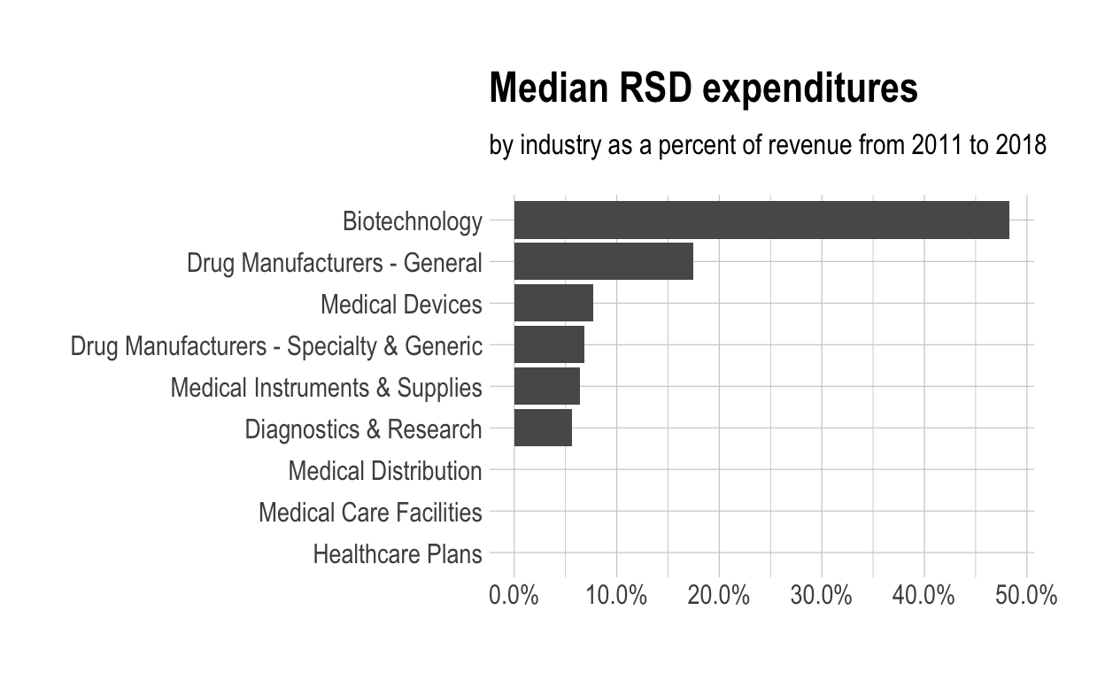
$ med_rnd_rev <dbl> 0.48317287, 0.05620271, 0.17451442, 0.06851879,…- Create a static bar chart.
ggplot(data = df,
       mapping = aes(
         x = reorder(industry, med_rnd_rev),
         y = med_rnd_rev
       )) +
geom_col() +
scale_y_continuous(labels = scales::percent) +
coord_flip() +
labs(
  title = "Median RSD expenditures",
  subtitle= "by industry as a percent of revenue from 2011 to 2018",
  x = NULL, y = NULL) +
theme_ipsum()
- Save the last plot to preview.png and add to the yaml chunk at the top
ggsave(filename = "preview.png", path = here::here("_posts", "2021-03-16-joining-data"))
- Create an interactive bar chart using the package
df %>%
  arrange(med_rnd_rev) %>%
  e_charts(
    x = industry
    ) %>%
  e_bar(
    serie = med_rnd_rev,
    name = "median"
    ) %>%
  e_flip_coords() %>%
  e_tooltip() %>%
  e_title(
    text = "Median industry R&D expenditures",
    subtext = "by industry as a percent of revenue from 2011 to 2018",
    left = "center") %>%
  e_legend(FALSE) %>%
  e_x_axis(
    formatter = e_axis_formatter("percent", digits = 0)
    ) %>%
  e_y_axis(
    show = FALSE
    ) %>%
  e_theme("infographic")